
Understanding StandardScaler: Why We Scale Input Features in Machine Learning
Published:
Understanding StandardScaler: Why We Scale Input Features in Machine Learning
1. Introduction
When building a machine learning model, the dataset usually contains many input features.
For example, in a student score prediction project, the input features may include:
age
study_hours
class_attendance
sleep_hours
These features do not always have the same range.
Example:
| Feature | Example Range |
|---|---|
age | 17 to 25 |
study_hours | 0 to 10 |
class_attendance | 0 to 100 |
sleep_hours | 3 to 10 |
The problem is that some features have much larger values than others.
For example:
age = 20
study_hours = 4.5
class_attendance = 85
sleep_hours = 7
The value 85 for class attendance is much larger than the value 4.5 for study hours.
However, this does not mean that class attendance is automatically much more important than study hours.
This is why we use feature scaling.
2. What Is Feature Scaling?
Feature scaling means changing the range of input features so that they are easier for the model to learn from.
In machine learning, we usually want the input features to be on a similar scale.
Without scaling, the model may train more slowly or may give too much attention to features with large numerical values.
For example, compare these two features:
study_hours = 4.5
class_attendance = 85
The attendance value is much larger, but the model should not assume it is more important only because the number is bigger.
Feature scaling solves this problem by transforming the values into a more balanced form.
3. What Is StandardScaler?
StandardScaler is a preprocessing tool from Scikit-learn.
It transforms each feature so that it has approximately:
mean = 0
standard deviation = 1
In Python, it is used like this:
from sklearn.preprocessing import StandardScaler

scaler = StandardScaler()
X_scaled = scaler.fit_transform(X)
The formula used by StandardScaler is:
Where:
| Symbol | Meaning |
|---|---|
| (x) | Original value |
| (\mu) | Mean of the feature |
| (\sigma) | Standard deviation of the feature |
| (z) | Standardized value, also called z-score |
In simple words:
standardized value = (original value - mean) / standard deviation
4. What Does the Formula Mean?
The formula is:
\[z = \frac{x - \mu}{\sigma}\]This formula tells us how far a value is from the average.
For example:
z = 0
means the value is exactly at the average.
z = 1
means the value is 1 standard deviation above the average.
z = -1
means the value is 1 standard deviation below the average.
z = 2
means the value is very high compared with the average.
z = -2
means the value is very low compared with the average.
5. Example: Scaling Class Attendance
Suppose the class attendance feature has:
mean = 70
standard deviation = 15
A student has:
class_attendance = 85
Using the StandardScaler formula:
\[z = \frac{85 - 70}{15}\] \[z = \frac{15}{15}\] \[z = 1\]So:
Original attendance = 85
Scaled attendance = 1
This means the student’s attendance is 1 standard deviation above the average.
6. Another Example: Low Attendance
Suppose another student has:
class_attendance = 55
Using the same mean and standard deviation:
\[z = \frac{55 - 70}{15}\] \[z = \frac{-15}{15}\] \[z = -1\]So:
Original attendance = 55
Scaled attendance = -1
This means the student’s attendance is 1 standard deviation below the average.
7. Simple Meaning of Z-Scores
After scaling, the values become easier to compare.
| Z-score | Meaning |
|---|---|
| -2 | Much lower than average |
| -1 | Lower than average |
| 0 | Average |
| 1 | Higher than average |
| 2 | Much higher than average |
So instead of comparing raw values like this:
age = 20
study_hours = 4.5
class_attendance = 85
sleep_hours = 7
The model may see scaled values like this:
age_scaled = 0.2
study_hours_scaled = 0.1
class_attendance_scaled = 1.0
sleep_hours_scaled = 0.4
Now the values are closer in scale, so the model can learn more smoothly.
8. Probability Graph Idea
StandardScaler is related to the idea of a standard normal distribution.
After standardization, the feature is centered around 0.
A standard normal distribution looks like this:
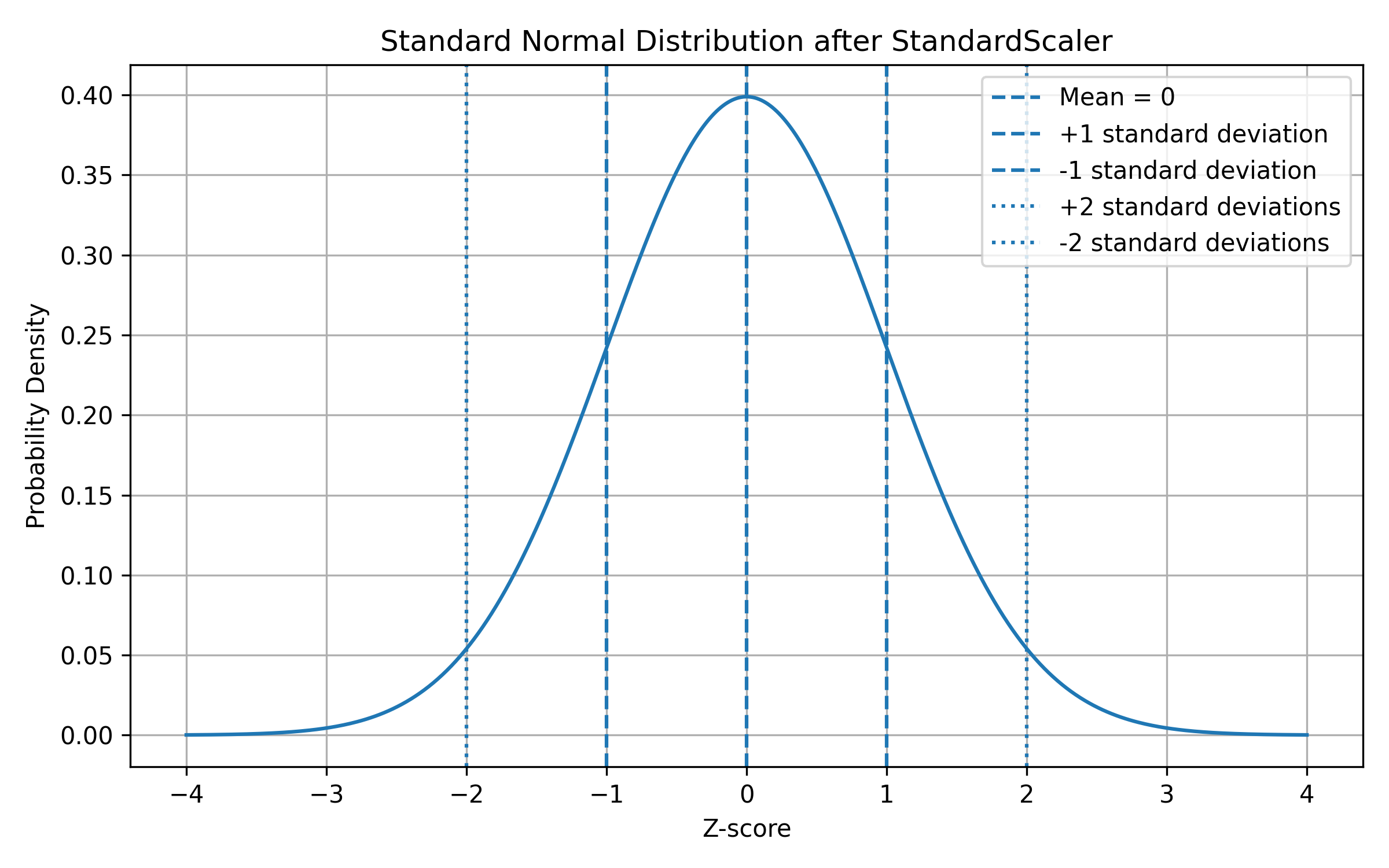
Most values are near the center.
Fewer values are far away from the center.
The center value is:
z = 0
This means average.
Values on the right side are above average:
z > 0
Values on the left side are below average:
z < 0
9. Explanation Under the Animation
The animation shows the transformation from the original value to the standardized value.
In this example:
class_attendance = 85
mean = 70
standard deviation = 15
Using the formula:
\[z = \frac{x - \mu}{\sigma}\]we get:
\[z = \frac{85 - 70}{15}\] \[z = 1\]This means that an attendance value of 85 is one standard deviation above the average.
After scaling, the model no longer sees the attendance value as 85. Instead, it sees the value as 1.
This helps the model compare attendance with other features such as age, study hours, and sleep hours.
11. Why Scaling Helps Machine Learning Models
Many machine learning models train using optimization.
In PyTorch, the model updates its weights using gradients.
If one feature has very large values and another feature has very small values, the gradient updates can become unbalanced.
For example, before scaling:
age = 20
study_hours = 4.5
class_attendance = 85
sleep_hours = 7
The value 85 is much larger than 4.5.
After scaling:
age_scaled ≈ 0.2
study_hours_scaled ≈ 0.1
class_attendance_scaled ≈ 1.0
sleep_hours_scaled ≈ 0.4
The values are now closer in range.
This helps the model train more smoothly.
12. Important Rule: Save the Scaler
When we use StandardScaler, we should save it after training.
Example:
joblib.dump(scaler, "student_scaler.pkl")
This is important because new input data must be scaled in exactly the same way as the training data.
The correct workflow is:
Training:
fit scaler on training data
scale training data
train model
save scaler

Prediction:
load saved scaler
scale new input using the same scaler
make prediction
The wrong workflow is:
Training:
scale training data

Prediction:
use raw unscaled input
If the model was trained on scaled data but prediction uses unscaled data, the prediction can become wrong.
13. Difference Between fit_transform() and transform()
This is one of the most important ideas.
During training, we use:
X = scaler.fit_transform(X)
During prediction, we use:
real_scaled = scaler.transform(real_input)
Training: fit_transform()
fit_transform() does two things:
1. fit: calculate mean and standard deviation from training data
2. transform: use those values to scale the training data
Prediction: transform()
transform() only scales the new data using the saved mean and standard deviation.
It does not calculate a new mean and standard deviation.
This is important because prediction data must follow the same scaling rule as training data.
14. Simple Summary
StandardScaler is used to put input features on a similar scale.
It uses the formula:
\[z = \frac{x - \mu}{\sigma}\]After scaling:
mean ≈ 0
standard deviation ≈ 1
This helps the model train more smoothly and prevents large-value features from dominating the learning process.
For the student score prediction project, scaling is useful because the input features have different ranges:
age: 17 to 25
study_hours: 0 to 10
class_attendance: 0 to 100
sleep_hours: 3 to 10
After scaling, the model learns from how far each value is from its average instead of learning from the raw number size.
This is why StandardScaler is an important preprocessing step in many machine learning projects.