
YOLOv8 Red & Green Object Detection Analysis
Published:
YOLOv8 Red & Green Object Detection
📌 Project Overview
This project uses YOLOv8 to detect and classify two object classes:
- 🟩
greenbox - 🟥
redbox
⚙️ Training Configuration
After running
yolo detect train model=yolov8n.pt data=data.yaml imgsz=320 epochs=10 batch=16 device=0
| Parameter | Value |
|---|---|
| Model | yolov8n |
| Image Size | 320 |
| Epochs | 10 |
| Batch Size | 16 |
| Device | GPU (device=0) |
📁 Important Output Files
Inside the training folder (runs/detect/train/), the most important files are:
results.png✅ (main training graph)confusion_matrix.png✅PR_curve.png✅F1_curve.png✅weights/best.pt✅
📊 results.png (Main Graph)
Shows:
- Training & validation loss
- Precision and recall
- mAP50 and mAP50-95
✔ What to check:
- Loss decreases over time → model is learning
- Validation follows training → no overfitting
- mAP increases → performance improves
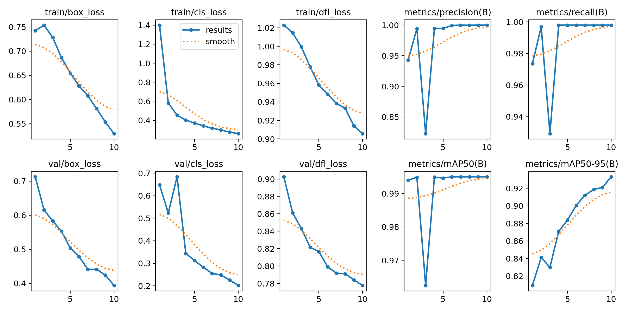
Throught the Graph we can analyze
1. TRAINING LOSS ANALYSIS
🔹 train/box_loss
- Decreases from ~0.75 → ~0.53
Smooth and consistent
Interpretation:
Model is improving bounding box localization
🔹 train/cls_loss
- Drops rapidly from ~1.4 → ~0.28
Interpretation: - Model quickly learns to classify
redboxvsgreenbox - Task is relatively easy (distinct colors)
🔹 train/dfl_loss
- Gradual decrease
Interpretation:
- Model is refining bounding box precision
2. Validation Loss Analysis
🔹 val/box_loss
- Smooth decrease
Interpretation:
- Good generalization to unseen validation data
🔹 val/cls_loss
- Spike at early epoch (~3)
- Then decreases steadily
Interpretation:
- Early training instability (normal)
- Model stabilizes afterward
🔹 val/dfl_loss
- Smooth decreasing trend
Interpretation:
- Bounding box quality improves on validation data
🚨 Key Concept: Overfitting Check
| Training Loss | Validation Loss | Meaning |
|---|---|---|
| ↓ | ↓ | ✅ Good (your case) |
| ↓ | ↑ | ❌ Overfitting |
| ↑ | ↑ | ❌ Poor training |
Conclusion:
- No overfitting observed
- Model generalizes well
3. Precision Analysis
- Starts ~0.94
- Drops briefly
- Converges to ~1.0
Interpretation:
- Very few false positives
- Temporary fluctuation is normal
4. Recall Analysis
- Similar behavior to precision
- Ends near 1.0
Interpretation:
- Model detects almost all objects
- Very few missed detections
📊 5. mAP Analysis (Most Important Metric)
🔹 mAP50
- Final value ≈ 0.995
Interpretation:
- Nearly perfect detection at IoU = 0.5
🔹 mAP50-95
- Improves from ~0.81 → ~0.93
Interpretation:
- Strong performance under stricter evaluation
- Indicates robust bounding box quality
⚠️ 6. Early Epoch Instability
Observed at epoch ~3:
- Drop in precision, recall, and mAP
Reason:
- Random weight initialization
- Learning adjustment phase
Important:
- This is normal behavior in training
- Focus on overall trend, not individual fluctuations
📉 7. Trend vs Raw Values
- Blue line: actual values
- Orange line: smoothed trend
Interpretation:
- Smoothed curve shows true learning behavior
- Model trend is stable and improving
📉 confusion_matrix.png
Shows classification performance:
| True \ Predicted | greenbox | redbox |
|---|---|---|
| greenbox | ✅ correct | ❌ wrong |
| redbox | ❌ wrong | ✅ correct |
What to check:
- Strong diagonal → good model
- Off-diagonal → classification errors
Below is the confusing matrix we get after the training
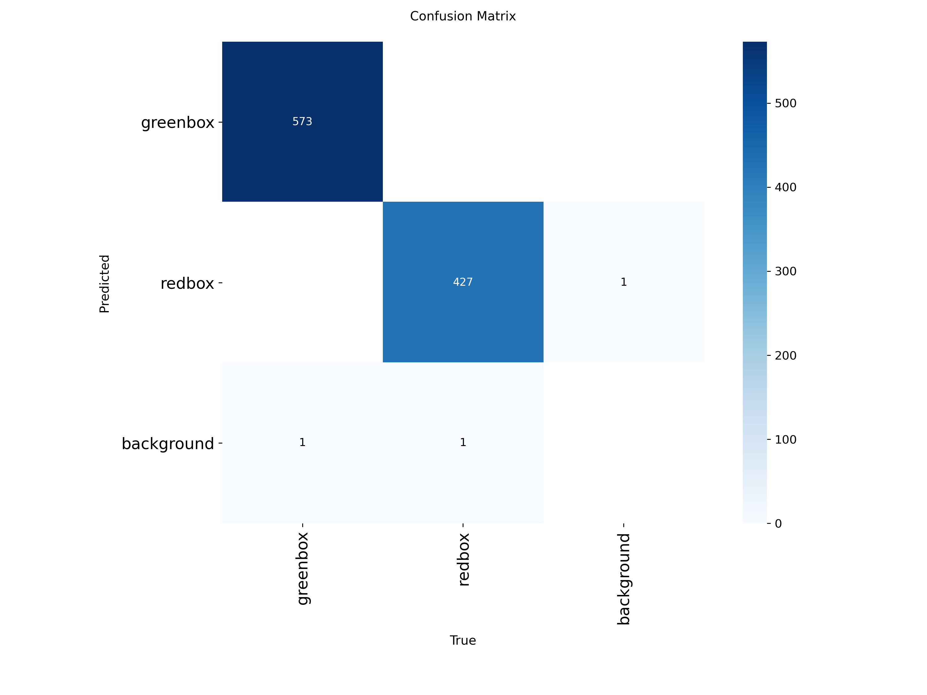
✅ Correct Predictions (Diagonal)
- greenbox → greenbox = 573
- redbox → redbox = 427
🎯 Interpretation:
- Model correctly classifies almost all objects
- Very strong diagonal → excellent performance
❌ Errors (Off-Diagonal)
🔹 False Positives (FP)
- 1 background detected as redbox
👉 Meaning:
- Model detected an object where there is none
🔹 False Negatives (FN)
- 1 greenbox missed (predicted as background)
- 1 redbox missed (predicted as background)
👉 Meaning:
- Model failed to detect some objects
📊 Error Summary
| Error Type | Count |
|---|---|
| False Positive | 1 |
| False Negative | 2 |
👉 Total errors = 3 (very low)
📈 Performance Interpretation
✅ Strengths
- Nearly perfect classification between red and green
- Almost no confusion between classes
- Extremely high accuracy
📈 PR_curve.png (Precision–Recall Curve)
Shows tradeoff between precision and recall.
What to check:
- Curve near top-right → excellent model
- Large area under curve → high performance
✅ 1. Precision–Recall (PR) Curve
Purpose:
- Shows overall model performance
- Combines:
- Precision (accuracy)
- Recall (completeness)
Why important:
- Used to compute mAP (main YOLO metric)
- Best indicator of model quality
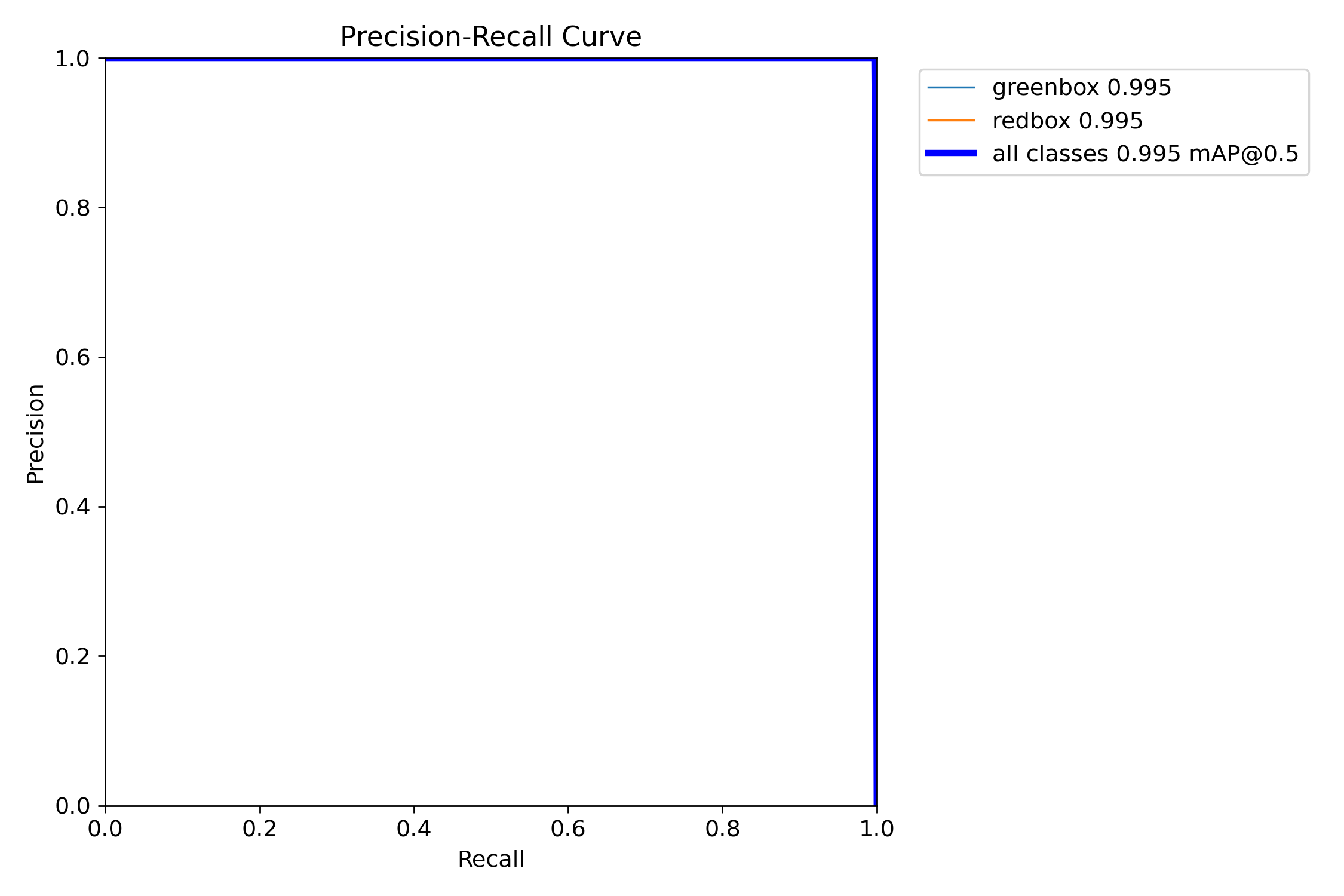
Result:
- Curve near top-right
- mAP ≈ 0.995
👉 Conclusion: Excellent model
📈 2. Precision–Confidence Curve (P Curve)
Purpose:
- Shows how precision changes with confidence threshold
Interpretation:
- Higher confidence → fewer false positives
- Model becomes more strict
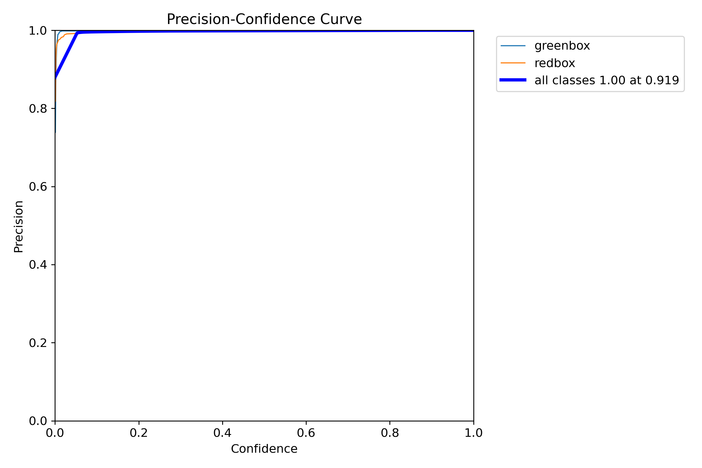
Result:
- Precision quickly reaches ~1.0
- Very stable
👉 Conclusion: Predictions are highly accurate
📉 3. Recall–Confidence Curve (R Curve)
Purpose:
- Shows how many objects are detected as threshold changes
Interpretation:
- Higher confidence → more missed detections
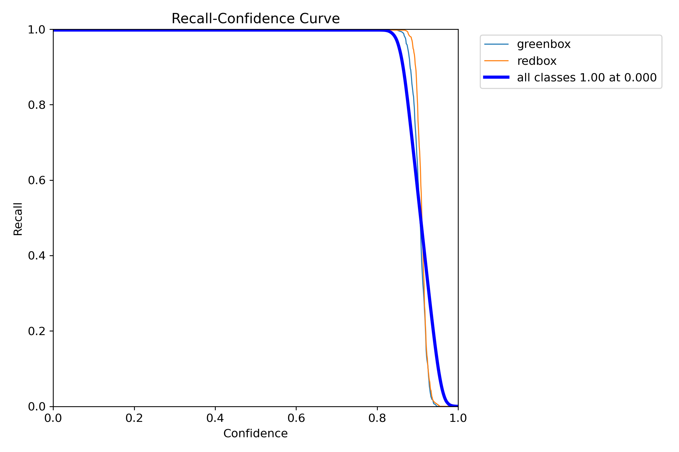
Result:
- Recall ≈ 1.0 at low confidence
- Drops sharply after ~0.9
👉 Conclusion: High confidence may miss objects
📊 F1_curve.png
Shows best balance between precision and recall.
What to check:
- Peak value → best performance
- Confidence at peak → optimal threshold
👉 It represents the best balance between Precision and Recall
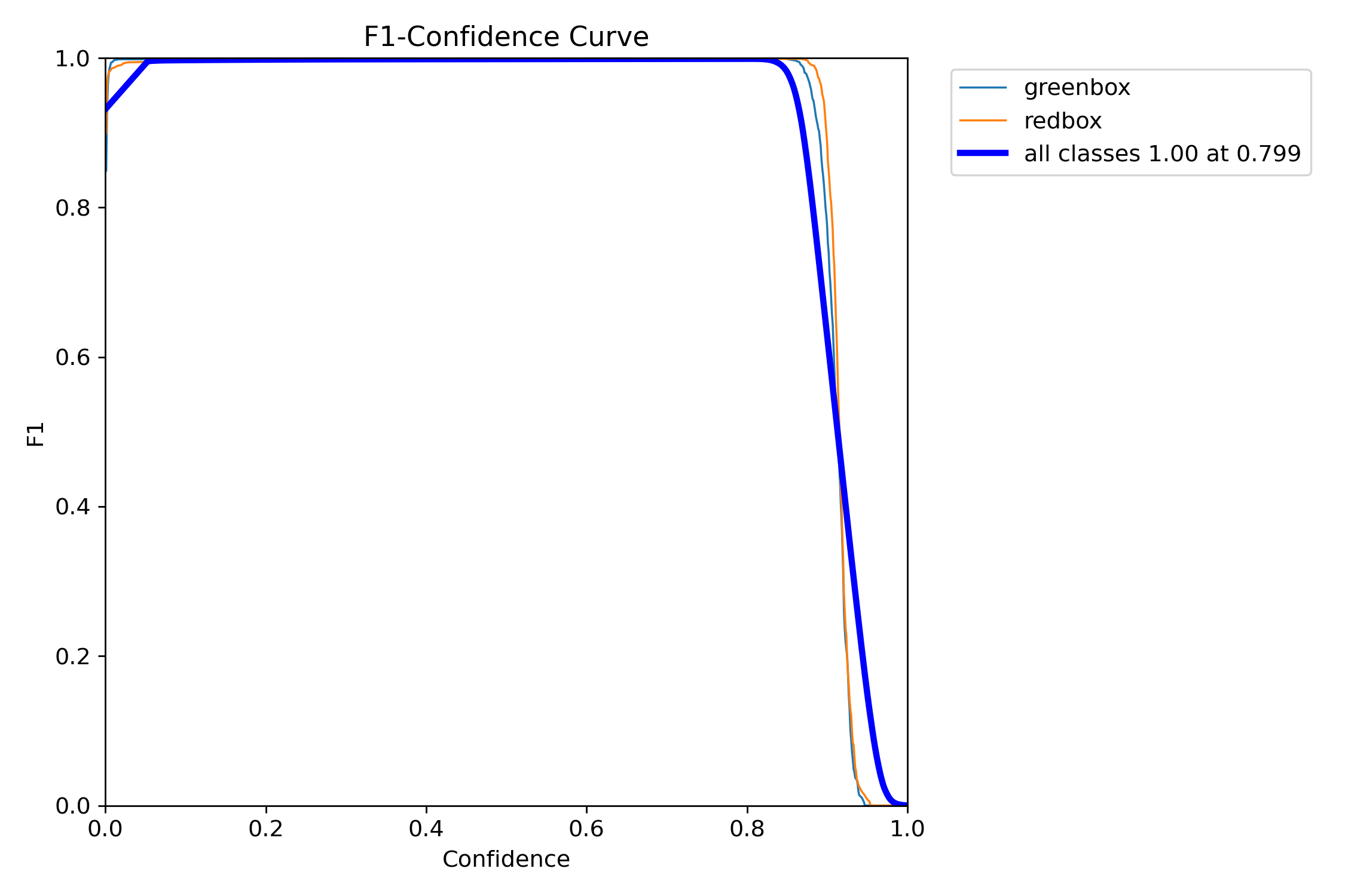
🔹 Shape:
- F1 is very high (~1.0) across a wide range
- Drops sharply after ~0.9 confidence
🔹 Key point:
- Best F1 ≈ 1.00 at confidence ≈ 0.799
✅ 1. Excellent Performance
- F1 ≈ 1.0 → almost perfect balance
- Means:
- Very few false positives
- Very few missed detections
👉 Model is extremely strong
⚖️ 2. Optimal Threshold
- Best confidence ≈ 0.8
👉 This is the ideal operating point
At this point:
- Precision is high
- Recall is high
- Overall performance is maximized
🧠 weights/best.pt
The final trained model.
Use it for inference:
yolo detect predict model=weights/best.pt source=your_image.jpg conf=0.8
1. Detection Output
For example:
yolo detect predict model=best.pt source=test/images/greenbox_0_jpg.rf.b7606581a957e3d3d3b8a36e5a4d82cb.jpg conf=0.8
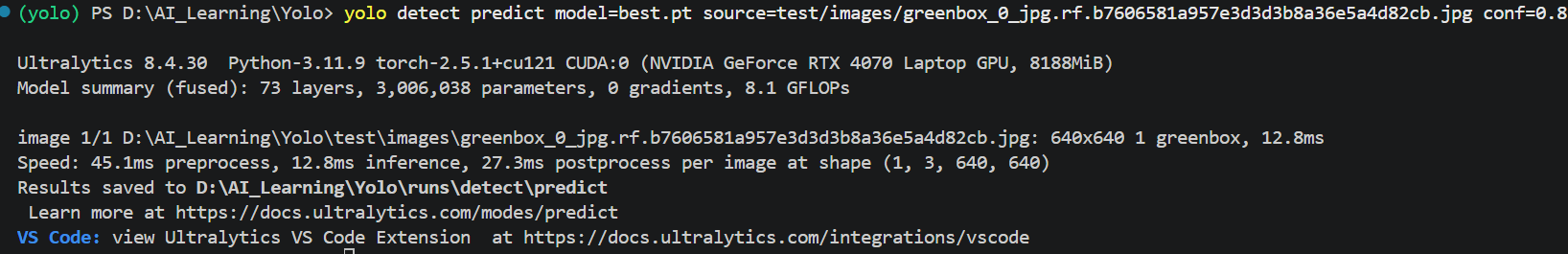
Model detected:
- 1 object
- Class = greenbox
- Inference time = 12.8 ms