
Breast Cancer Classification using PyTorch: A Complete Binary Classification Project
Published:
Breast Cancer Classification using PyTorch: A Complete Binary Classification Project
1. Introduction
In the previous PyTorch lesson, we used a simple linear regression model to predict a continuous value.
For example:
Input:
study_hours
class_attendance
sleep_hours

Output:
student_score
That project was a regression problem because the output was a number.
In this project, we move to a new type of machine learning problem:
Binary Classification
The goal is to predict one of two possible classes.
In this project, we use the Breast Cancer Wisconsin Dataset to predict whether a tumor is:
0 = Malignant
1 = Benign
This project is useful because it shows a complete PyTorch workflow:
load dataset
prepare data
scale features
split train and test data
convert data to PyTorch tensors
create DataLoader
build neural network
train the model
evaluate the model
plot training loss
plot confusion matrix
plot ROC curve
save the model
load the model
predict unknown data
This article focuses on the project explanation.
The basic concepts such as neural networks, tensors, StandardScaler, and binary classification are already explained in the previous articles.
2. Project Goal
The main goal of this project is:
Given 30 tumor measurements,
predict whether the tumor is malignant or benign.
The model receives input features such as:
mean radius
mean texture
mean perimeter
mean area
mean smoothness
Then it predicts one output:
0 or 1
The target meaning is:
| Target Value | Meaning |
|---|---|
| 0 | Malignant |
| 1 | Benign |
In simple words:
Malignant = cancerous tumor
Benign = non-cancerous tumor
3. Dataset Overview
We use the dataset directly from Scikit-learn:
from sklearn.datasets import load_breast_cancer
This dataset contains measurements from breast tumor samples.
The dataset has:
| Item | Value |
|---|---|
| Number of samples | 569 |
| Number of input features | 30 |
| Number of classes | 2 |
The target distribution is:
1    357
0    212
This means:
357 benign tumors
212 malignant tumors
So the dataset is not perfectly balanced, but it is still acceptable for a beginner binary classification project.
4. Project Workflow
The full workflow is:
Breast Cancer Dataset
        ↓
Create X and y
        ↓
Scale input features
        ↓
Split train/test data
        ↓
Convert to PyTorch tensors
        ↓
Create TensorDataset
        ↓
Create DataLoader
        ↓
Build neural network
        ↓
Train model
        ↓
Evaluate model
        ↓
Save model
        ↓
Predict unknown patient
In this project, I separated the code into three files:
data_prep.py
train_binary.py
predict.py
The purpose of each file is:
| File | Purpose |
|---|---|
data_prep.py | Load and prepare the dataset |
train_binary.py | Train and evaluate the PyTorch model |
predict.py | Load the saved model and predict unknown data |
5. Data Preparation File: data_prep.py
The first file prepares the data before training.
Full code:
#%% Packages
import pandas as pd
import joblib

from sklearn.datasets import load_breast_cancer
from sklearn.model_selection import train_test_split
from sklearn.preprocessing import StandardScaler

# =============================================================================
# LOAD DATASET
# =============================================================================

data = load_breast_cancer()

X = pd.DataFrame(
    data.data,
    columns=data.feature_names
)

y = pd.Series(
    data.target,
    name="target"
)

print("\nDataset Shape")
print(X.shape)

print("\nFeature Names")
print(X.columns.tolist())

print("\nTarget Distribution")
print(y.value_counts())

# =============================================================================
# FEATURE SCALING
# =============================================================================

scaler = StandardScaler()

X_scaled = scaler.fit_transform(X)

joblib.dump(
    scaler,
    "scaler.pkl"
)

# =============================================================================
# TRAIN TEST SPLIT
# =============================================================================

X_train, X_test, y_train, y_test = train_test_split(
    X_scaled,
    y,
    test_size=0.2,
    stratify=y,
    random_state=42
)

print("\nTrain/Test Split")
print(f"X_train: {X_train.shape}")
print(f"X_test : {X_test.shape}")
6. Explaining the Data Preparation Code
6.1 Import Packages
import pandas as pd
import joblib
pandas is used to create a table-like dataset.
joblib is used to save the StandardScaler object.
We save the scaler because future unknown data must be scaled using the same mean and standard deviation as the training data.
6.2 Load the Dataset
data = load_breast_cancer()
This loads the breast cancer dataset from Scikit-learn.
The object data contains:
data.data
data.target
data.feature_names
data.target_names
6.3 Create the Feature Matrix X
X = pd.DataFrame(
    data.data,
    columns=data.feature_names
)
X contains the input features.
Each row represents one tumor sample.
Each column represents one measurement.
For example:
mean radius
mean texture
mean perimeter
mean area
mean smoothness
The shape is:
(569, 30)
This means:
569 samples
30 input features
6.4 Create the Target Vector y
y = pd.Series(
    data.target,
    name="target"
)
y contains the correct answer for each sample.
The values are:
0 = malignant
1 = benign
So for each row in X, there is one matching label in y.
Example:
| Tumor sample | Features | Target |
|---|---|---|
| Sample 1 | 30 measurements | 0 |
| Sample 2 | 30 measurements | 1 |
| Sample 3 | 30 measurements | 1 |
6.5 Print Dataset Information
print(X.shape)
print(X.columns.tolist())
print(y.value_counts())
This helps us understand the dataset before training.
The output is similar to:
Dataset Shape
(569, 30)

Target Distribution
1    357
0    212
This tells us:
There are 569 total samples.
There are 30 input features.
There are 357 benign tumors.
There are 212 malignant tumors.
7. Feature Scaling
The model should not train directly on raw input values.
Some features may have values like:
mean radius = 14
mean area = 650
worst area = 850
The area values are much larger than radius values.
If we train directly on these raw numbers, the model may give too much attention to features with large values.
So we use:
scaler = StandardScaler()

X_scaled = scaler.fit_transform(X)
StandardScaler changes the data so that each feature has approximately:
mean = 0
standard deviation = 1
This helps the model train more smoothly.
8. Saving the Scaler
joblib.dump(
    scaler,
    "scaler.pkl"
)
This saves the fitted scaler.
This is very important.
During training, we use:
fit_transform()
This calculates the mean and standard deviation from the training data.
During prediction, we must use:
transform()
This uses the same mean and standard deviation.
The correct workflow is:
Training:
fit scaler
scale training data
save scaler

Prediction:
load scaler
scale unknown data
predict using trained model
If we do not save the scaler, unknown data may be scaled differently, and the prediction may become wrong.
9. Train/Test Split
X_train, X_test, y_train, y_test = train_test_split(
    X_scaled,
    y,
    test_size=0.2,
    stratify=y,
    random_state=42
)
This separates the dataset into training and testing data.
Training data = used for learning
Testing data = used for final evaluation
Because test_size=0.2, the data is split into:
80% training
20% testing
The output is:
X_train: (455, 30)
X_test : (114, 30)
This means:
455 samples are used for training.
114 samples are used for testing.
10. Why Use stratify=y?
stratify=y
This keeps the class distribution similar in both training and testing sets.
Original dataset:
357 benign
212 malignant
If we split randomly without stratify, the test set might accidentally contain too many benign or too many malignant samples.
With stratify=y, the train and test sets keep a similar class ratio.
This makes evaluation fairer.
11. Training File: train_binary.py
After preparing the data, we train the PyTorch model.
Full code:
#%% Packages
import torch
import torch.nn as nn
import torch.optim as optim

from torch.utils.data import (
    TensorDataset,
    DataLoader
)

import matplotlib.pyplot as plt
import seaborn as sns

from sklearn.metrics import (
    confusion_matrix,
    accuracy_score,
    classification_report,
    roc_curve,
    auc
)

from sklearn.dummy import DummyClassifier

from data_prep import (
    X_train,
    X_test,
    y_train,
    y_test
)

# =============================================================================
# HYPERPARAMETERS
# =============================================================================

BATCH_SIZE = 16
LEARNING_RATE = 0.001
EPOCHS = 50

DEVICE = torch.device(
    "cuda" if torch.cuda.is_available() else "cpu"
)

print("Device:", DEVICE)

# =============================================================================
# DATASET
# =============================================================================

train_dataset = TensorDataset(
    torch.tensor(X_train, dtype=torch.float32),
    torch.tensor(y_train.values, dtype=torch.float32)
)

test_dataset = TensorDataset(
    torch.tensor(X_test, dtype=torch.float32),
    torch.tensor(y_test.values, dtype=torch.float32)
)

train_loader = DataLoader(
    train_dataset,
    batch_size=BATCH_SIZE,
    shuffle=True
)

test_loader = DataLoader(
    test_dataset,
    batch_size=BATCH_SIZE,
    shuffle=False
)

# =============================================================================
# MODEL
# =============================================================================

class BreastCancerModel(nn.Module):

    def __init__(self, input_size):

        super().__init__()

        self.network = nn.Sequential(

            nn.Linear(input_size, 32),
            nn.ReLU(),

            nn.Linear(32, 16),
            nn.ReLU(),

            nn.Linear(16, 1)

        )

    def forward(self, x):
        return self.network(x)

# =============================================================================
# CREATE MODEL
# =============================================================================

INPUT_SIZE = X_train.shape[1]

model = BreastCancerModel(
    input_size=INPUT_SIZE
).to(DEVICE)

print(model)

# =============================================================================
# LOSS FUNCTION
# =============================================================================

loss_fn = nn.BCEWithLogitsLoss()

optimizer = optim.Adam(
    model.parameters(),
    lr=LEARNING_RATE
)

# =============================================================================
# TRAINING
# =============================================================================

train_losses = []

for epoch in range(EPOCHS):

    model.train()

    running_loss = 0

    for X_batch, y_batch in train_loader:

        X_batch = X_batch.to(DEVICE)
        y_batch = y_batch.to(DEVICE)

        optimizer.zero_grad()

        logits = model(X_batch)

        loss = loss_fn(
            logits,
            y_batch.view(-1,1)
        )

        loss.backward()

        optimizer.step()

        running_loss += loss.item()

    avg_loss = running_loss / len(train_loader)

    train_losses.append(avg_loss)

    print(
        f"Epoch [{epoch+1:02d}/{EPOCHS}] "
        f"Loss: {avg_loss:.4f}"
    )

# =============================================================================
# LOSS CURVE
# =============================================================================

plt.figure(figsize=(8,5))

plt.plot(
    range(1,EPOCHS+1),
    train_losses,
    marker='o'
)

plt.xlabel("Epoch")
plt.ylabel("Loss")
plt.title("Training Loss")
plt.grid()

plt.savefig(
    "breast_cancer_training_loss.png",
    dpi=300,
    bbox_inches="tight"
)

plt.show()

# =============================================================================
# EVALUATION
# =============================================================================

model.eval()

y_true = []
y_pred = []
y_prob = []

with torch.no_grad():

    for X_batch, y_batch in test_loader:

        X_batch = X_batch.to(DEVICE)

        logits = model(X_batch)

        probabilities = torch.sigmoid(logits)

        predictions = (
            probabilities > 0.5
        ).int()

        y_true.extend(
            y_batch.numpy()
        )

        y_pred.extend(
            predictions.cpu().numpy().flatten()
        )

        y_prob.extend(
            probabilities.cpu().numpy().flatten()
        )

# =============================================================================
# ACCURACY
# =============================================================================

accuracy = accuracy_score(
    y_true,
    y_pred
)

print("\nAccuracy")
print(accuracy)

# =============================================================================
# REPORT
# =============================================================================

print("\nClassification Report")

print(
    classification_report(
        y_true,
        y_pred
    )
)

# =============================================================================
# CONFUSION MATRIX
# =============================================================================

cm = confusion_matrix(
    y_true,
    y_pred
)

plt.figure(figsize=(6,5))

sns.heatmap(
    cm,
    annot=True,
    fmt='d',
    cmap='Blues'
)

plt.xlabel("Predicted")
plt.ylabel("Actual")
plt.title("Confusion Matrix")

plt.savefig(
    "breast_cancer_confusion_matrix.png",
    dpi=300,
    bbox_inches="tight"
)

plt.show()

# =============================================================================
# ROC CURVE
# =============================================================================

fpr, tpr, thresholds = roc_curve(
    y_true,
    y_prob
)

roc_auc = auc(
    fpr,
    tpr
)

plt.figure(figsize=(8,6))

plt.plot(
    fpr,
    tpr,
    label=f"AUC = {roc_auc:.4f}"
)

plt.plot(
    [0,1],
    [0,1],
    '--'
)

plt.xlabel("False Positive Rate")
plt.ylabel("True Positive Rate")
plt.title("ROC Curve")

plt.legend()
plt.grid()

plt.savefig(
    "breast_cancer_roc_curve.png",
    dpi=300,
    bbox_inches="tight"
)

plt.show()

print("\nAUC Score")
print(roc_auc)

# =============================================================================
# BASELINE
# =============================================================================

baseline = DummyClassifier(
    strategy="most_frequent"
)

baseline.fit(
    X_train,
    y_train
)

baseline_pred = baseline.predict(
    X_test
)

baseline_acc = accuracy_score(
    y_test,
    baseline_pred
)

print("\nBaseline Accuracy")
print(baseline_acc)

print("\nNeural Network Accuracy")
print(accuracy)

# =============================================================================
# SAVE MODEL
# =============================================================================

torch.save(
    model.state_dict(),
    "breast_cancer_model.pth"
)

print("\nModel saved successfully!")
12. Importing PyTorch Packages
import torch
import torch.nn as nn
import torch.optim as optim
These are the main PyTorch packages.
| Package | Purpose |
|---|---|
torch | Tensor operations |
torch.nn | Neural network layers |
torch.optim | Optimizers such as Adam |
13. Importing Dataset Tools
from torch.utils.data import (
    TensorDataset,
    DataLoader
)
TensorDataset combines input tensors and target tensors.
DataLoader helps the model train using mini-batches.
Instead of giving all 455 training samples to the model at once, DataLoader gives smaller groups of samples.
14. Hyperparameters
BATCH_SIZE = 16
LEARNING_RATE = 0.001
EPOCHS = 50
These are training settings.
Batch Size
BATCH_SIZE = 16
This means the model trains with 16 samples at a time.
Because there are 455 training samples:
455 / 16 ≈ 28.4
So one epoch has about 29 mini-batches.
One epoch means the model sees all 455 training samples once.
Epochs
EPOCHS = 50
This means the model will go through the whole training dataset 50 times.
Learning Rate
LEARNING_RATE = 0.001
The learning rate controls how large each weight update is.
A small learning rate learns slowly but safely.
A large learning rate learns faster but may overshoot the best solution.
15. CPU or GPU
DEVICE = torch.device(
    "cuda" if torch.cuda.is_available() else "cpu"
)
This checks whether GPU is available.
If CUDA is available, the model uses GPU.
Otherwise, it uses CPU.
Output:
Device: cpu
This means the training runs on the CPU.
For this dataset, CPU is fine because the dataset is small.
16. Creating PyTorch Dataset
train_dataset = TensorDataset(
    torch.tensor(X_train, dtype=torch.float32),
    torch.tensor(y_train.values, dtype=torch.float32)
)
PyTorch models cannot train directly on Pandas or NumPy data.
So we convert the data into tensors.
Each sample becomes:
(input_features, target)
Example:
[0.21, -0.52, 1.33, ...] → 1
The first tensor contains the input features.
The second tensor contains the correct label.
17. Creating DataLoader
train_loader = DataLoader(
    train_dataset,
    batch_size=BATCH_SIZE,
    shuffle=True
)
The DataLoader splits the training dataset into mini-batches.
Because batch_size=16, each batch contains 16 samples.
shuffle=True means the order of training samples is randomly changed each epoch.
This helps the model learn better because it does not always see the samples in the same order.
For the test loader:
test_loader = DataLoader(
    test_dataset,
    batch_size=BATCH_SIZE,
    shuffle=False
)
We use shuffle=False because we are only evaluating the model.
18. Neural Network Model
class BreastCancerModel(nn.Module):
This defines a custom PyTorch model.
The architecture is:
30 input features
        ↓
32 neurons
        ↓
16 neurons
        ↓
1 output
The code is:
self.network = nn.Sequential(

    nn.Linear(input_size, 32),
    nn.ReLU(),

    nn.Linear(32, 16),
    nn.ReLU(),

    nn.Linear(16, 1)

)
19. Linear Layers
nn.Linear(input_size, 32)
The first layer receives 30 input features and produces 32 outputs.
Because:
INPUT_SIZE = X_train.shape[1]
and X_train.shape[1] is 30.
So the first layer is:
Linear(30 → 32)
The second layer is:
Linear(32 → 16)
The final layer is:
Linear(16 → 1)
The final output is one number because this is binary classification.
20. ReLU Activation
nn.ReLU()
ReLU helps the neural network learn non-linear patterns.
Without activation functions, multiple linear layers would still behave like one linear layer.
ReLU changes negative values to zero and keeps positive values.
ReLU(-5) = 0
ReLU(3) = 3
21. Output Layer and Logits
The final layer outputs one raw number.
This raw number is called a logit.
Example:
logit = 4.5
logit = -2.1
logit = 0.3
A positive logit usually means the model leans toward class 1.
A negative logit usually means the model leans toward class 0.
But logits are not probabilities yet.
To convert logits into probabilities, we use sigmoid during evaluation:
probabilities = torch.sigmoid(logits)
22. Loss Function
loss_fn = nn.BCEWithLogitsLoss()
This loss function is used for binary classification.
It combines two steps:
sigmoid
binary cross entropy loss
We do not put sigmoid inside the model during training because BCEWithLogitsLoss() already includes sigmoid internally.
This is more numerically stable.
23. Optimizer
optimizer = optim.Adam(
    model.parameters(),
    lr=LEARNING_RATE
)
The optimizer updates the model weights.
The model first makes predictions.
Then the loss function measures the error.
Then backpropagation calculates gradients.
Then Adam updates the weights to reduce the loss.
The learning rate controls how large the update is.
24. Training Loop
The training loop is the heart of the project.
for epoch in range(EPOCHS):
This repeats the training process 50 times.
Inside each epoch:
model.train()
This sets the model to training mode.
Then:
running_loss = 0
This stores the total loss for the epoch.
24.1 Loop Through Mini-Batches
for X_batch, y_batch in train_loader:
This takes one mini-batch at a time.
Because batch size is 16, each batch contains 16 samples.
For each mini-batch, the model does:
forward pass
loss calculation
backward pass
weight update
24.2 Move Batch to Device
X_batch = X_batch.to(DEVICE)
y_batch = y_batch.to(DEVICE)
If the model is on GPU, the data must also be on GPU.
If the model is on CPU, the data stays on CPU.
The model and the data must be on the same device.
24.3 Clear Old Gradients
optimizer.zero_grad()
PyTorch accumulates gradients by default.
So before calculating new gradients, we clear the old gradients.
If we forget this line, gradients from previous batches will mix with gradients from the current batch.
This can make training incorrect.
24.4 Forward Pass
logits = model(X_batch)
The model receives the input batch and produces logits.
For example:
Input batch: 16 tumor samples
Output: 16 logits
Each logit is one raw prediction.
24.5 Calculate Loss
loss = loss_fn(
    logits,
    y_batch.view(-1,1)
)
This compares the predicted logits with the true labels.
The target y_batch is reshaped using:
y_batch.view(-1,1)
This makes the target shape match the output shape.
If the model output shape is:
[16, 1]
then the target should also be:
[16, 1]
24.6 Backpropagation
loss.backward()
This calculates gradients.
A gradient tells the model how each weight should change to reduce the loss.
In simple words:
loss.backward()
= calculate how wrong each weight was
24.7 Update Weights
optimizer.step()
This updates the model weights using the gradients.
This is where learning actually happens.
The weight update happens after every mini-batch, not only after each epoch.
Because there are about 29 mini-batches per epoch and 50 epochs:
29 × 50 = 1450 weight updates
So the model updates its weights around 1450 times.
24.8 Store the Loss
running_loss += loss.item()
This adds the current batch loss to the total epoch loss.
Then:
avg_loss = running_loss / len(train_loader)
calculates the average loss for that epoch.
This is what we print.
25. Training Output
Example output:
Epoch [01/50] Loss: 0.6512
Epoch [02/50] Loss: 0.4548
Epoch [03/50] Loss: 0.2650
Epoch [04/50] Loss: 0.1629
Epoch [05/50] Loss: 0.1127
Epoch [10/50] Loss: 0.0529
Epoch [20/50] Loss: 0.0282
Epoch [30/50] Loss: 0.0154
Epoch [40/50] Loss: 0.0082
Epoch [50/50] Loss: 0.0043
This shows that the model is learning.
At the beginning:
Loss = 0.6512
The model is still weak.
After a few epochs:
Loss = 0.1127
The model has learned many useful patterns.
At the end:
Loss = 0.0043
The model fits the training data very well.
26. Training Loss Graph
The training loss graph shows how the loss changes over epochs.
The graph is saved using:
plt.savefig(
    "breast_cancer_training_loss.png",
    dpi=300,
    bbox_inches="tight"
)
Example:
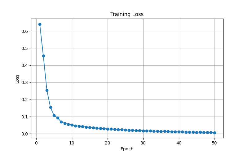
The expected shape is:
high loss at the beginning
fast decrease in the first few epochs
slow decrease later
almost flat near the end
This is a healthy training curve.
It means the model learned quickly in the beginning and then slowly fine-tuned the weights.
27. Evaluation Mode
After training, we evaluate the model.
model.eval()
This tells PyTorch that the model is no longer training.
During evaluation:
no weight update
no dropout behavior
no training-specific behavior
Even though this model does not use dropout, using model.eval() is still good practice.
28. Disable Gradient Calculation
with torch.no_grad():
During evaluation, we do not need gradients.
We only need predictions.
Using torch.no_grad():
saves memory
makes prediction faster
prevents accidental gradient calculation
29. Sigmoid and Threshold
During evaluation:
probabilities = torch.sigmoid(logits)
This converts logits into probabilities.
Example:
logit = 5
sigmoid(logit) = 0.993
Then:
predictions = (
    probabilities > 0.5
).int()
This converts probability into class label.
probability > 0.5  → class 1
probability <= 0.5 → class 0
For this dataset:
class 1 = benign
class 0 = malignant
30. Accuracy
accuracy = accuracy_score(
    y_true,
    y_pred
)
Accuracy means:
correct predictions / total predictions
Example result:
Accuracy
0.956140350877193
This means the model predicted correctly about:
95.61% of the time
31. Classification Report
Example output:
Classification Report
              precision    recall  f1-score   support

         0.0       0.91      0.98      0.94        42
         1.0       0.99      0.94      0.96        72

    accuracy                           0.96       114
   macro avg       0.95      0.96      0.95       114
weighted avg       0.96      0.96      0.96       114
Class meaning:
0 = malignant
1 = benign
For class 0:
precision = 0.91
recall = 0.98
f1-score = 0.94
support = 42
This means there were 42 malignant samples in the test set.
The model detected almost all malignant cases because recall is 0.98.
This is important because missing malignant tumors would be dangerous.
For class 1:
precision = 0.99
recall = 0.94
f1-score = 0.96
support = 72
This means there were 72 benign samples in the test set.
The model also performed very well on benign cases.
32. Confusion Matrix
The confusion matrix is created using:
cm = confusion_matrix(
    y_true,
    y_pred
)
Then plotted using seaborn:
sns.heatmap(
    cm,
    annot=True,
    fmt='d',
    cmap='Blues'
)
Example:
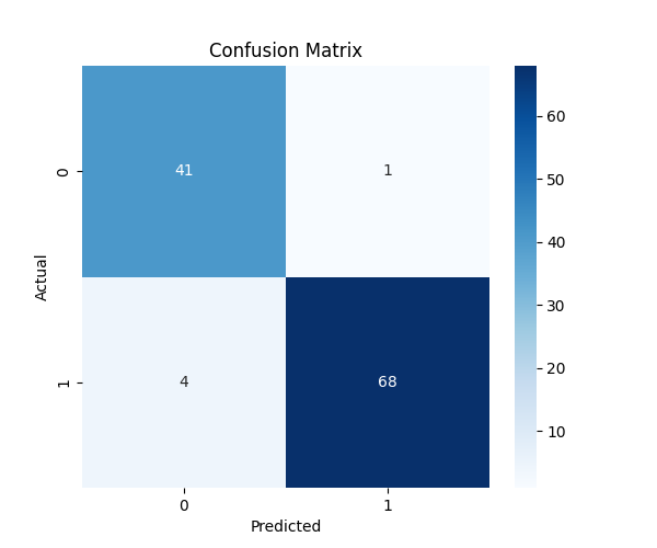
A confusion matrix shows:
what the true class was
what the model predicted
For binary classification, it looks like:
| Predicted 0 | Predicted 1 | |
|---|---|---|
| Actual 0 | Correct malignant | Malignant predicted as benign |
| Actual 1 | Benign predicted as malignant | Correct benign |
This is more useful than accuracy alone because it shows exactly where the model makes mistakes.
33. ROC Curve
The ROC curve is created using:
fpr, tpr, thresholds = roc_curve(
    y_true,
    y_prob
)
The AUC score is calculated using:
roc_auc = auc(
    fpr,
    tpr
)
Then the graph is saved using:
plt.savefig(
    "breast_cancer_roc_curve.png",
    dpi=300,
    bbox_inches="tight"
)
Example:
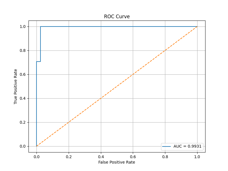
The ROC curve shows how well the model separates the two classes.
A random model has an AUC around:
0.5
A perfect model has an AUC of:
1.0
Example result:
AUC Score
0.9920634920634921
This is very high.
It means the model is very good at separating malignant and benign samples.
34. Baseline Model
A baseline model is a simple model used for comparison.
baseline = DummyClassifier(
    strategy="most_frequent"
)
This model always predicts the most common class.
In this dataset, the most common class is benign.
So the baseline model predicts:
everything = benign
The baseline result is:
Baseline Accuracy
0.631578947368421
This means if we always predict the most common class, we get about:
63.16% accuracy
The PyTorch neural network result is:
Neural Network Accuracy
0.956140350877193
This means the neural network performs much better than the baseline.
35. Saving the Model
After training, we save the model:
torch.save(
    model.state_dict(),
    "breast_cancer_model.pth"
)
This saves the learned weights.
It does not save the entire Python class.
That is why, when loading the model later, we must define the same model architecture again.
The saved file is:
breast_cancer_model.pth
This file contains the knowledge learned by the model.
36. Prediction File: predict.py
After training, we can use the saved model to predict unknown data.
Full code:
import torch
import torch.nn as nn
import joblib
import pandas as pd

# =============================================================================
# MODEL DEFINITION
# =============================================================================

class BreastCancerModel(nn.Module):

    def __init__(self, input_size):

        super().__init__()

        self.network = nn.Sequential(

            nn.Linear(input_size, 32),
            nn.ReLU(),

            nn.Linear(32, 16),
            nn.ReLU(),

            nn.Linear(16, 1)

        )

    def forward(self, x):
        return self.network(x)

# =============================================================================
# LOAD SCALER
# =============================================================================

scaler = joblib.load(
    "scaler.pkl"
)

# =============================================================================
# LOAD MODEL
# =============================================================================

INPUT_SIZE = 30

model = BreastCancerModel(
    INPUT_SIZE
)

model.load_state_dict(
    torch.load(
        "breast_cancer_model.pth",
        map_location="cpu"
    )
)

model.eval()

print("Model loaded successfully!")

# =============================================================================
# UNKNOWN PATIENT DATA
# =============================================================================

new_patient = [

    14.2,
    18.5,
    92.1,
    650.0,
    0.10,
    0.12,
    0.09,
    0.05,
    0.18,
    0.06,

    0.40,
    1.20,
    2.50,
    30.0,
    0.006,
    0.020,
    0.030,
    0.010,
    0.020,
    0.003,

    16.0,
    25.0,
    105.0,
    850.0,
    0.14,
    0.30,
    0.40,
    0.15,
    0.30,
    0.08
]

# =============================================================================
# CREATE DATAFRAME WITH FEATURE NAMES
# =============================================================================

new_patient_df = pd.DataFrame(
    [new_patient],
    columns=scaler.feature_names_in_
)

# =============================================================================
# SCALE DATA
# =============================================================================

new_patient_scaled = scaler.transform(
    new_patient_df
)

# =============================================================================
# CONVERT TO TENSOR
# =============================================================================

tensor = torch.tensor(
    new_patient_scaled,
    dtype=torch.float32
)

# =============================================================================
# PREDICTION
# =============================================================================

with torch.no_grad():

    logits = model(tensor)

    probability = torch.sigmoid(logits)

    probability = probability.item()

# =============================================================================
# RESULT
# =============================================================================

print("\nPrediction Probability")
print(f"{probability:.4f}")

print(f"Benign Probability: {probability:.4f}")
print(f"Malignant Probability: {1 - probability:.4f}")

if probability > 0.5:

    print("Prediction: BENIGN")

else:

    print("Prediction: MALIGNANT")
37. Why Load the Scaler?
scaler = joblib.load(
    "scaler.pkl"
)
The model was trained using scaled data.
So unknown data must also be scaled before prediction.
If the model was trained on scaled data but we give it raw data, the prediction can become incorrect.
This is one of the most common mistakes in machine learning deployment.
38. Why Define the Model Again?
class BreastCancerModel(nn.Module):
When we save using:
torch.save(model.state_dict(), "breast_cancer_model.pth")
we only save the weights.
We do not save the class definition.
So in predict.py, we must recreate the same architecture:
30 → 32 → 16 → 1
Then we load the saved weights into it.
39. Loading the Model Weights
model.load_state_dict(
    torch.load(
        "breast_cancer_model.pth",
        map_location="cpu"
    )
)
This loads the learned weights into the model.
map_location="cpu" makes sure the model loads correctly even if it was trained on GPU but predicted on CPU.
40. Why Use a DataFrame for Unknown Data?
new_patient_df = pd.DataFrame(
    [new_patient],
    columns=scaler.feature_names_in_
)
This prevents the warning:
X does not have valid feature names, but StandardScaler was fitted with feature names
The scaler was fitted using a DataFrame with column names.
So during prediction, we also provide a DataFrame with the same feature names.
41. Scale Unknown Data
new_patient_scaled = scaler.transform(
    new_patient_df
)
We use transform() instead of fit_transform().
During prediction, we do not calculate a new mean and standard deviation.
We use the saved mean and standard deviation from training.
42. Make Prediction
logits = model(tensor)

probability = torch.sigmoid(logits)

probability = probability.item()
The model first gives a logit.
Then sigmoid converts the logit into a probability.
Then .item() converts the one-value tensor into a normal Python number.
43. Interpreting the Prediction
Example output:
Model loaded successfully!

Prediction Probability
0.0035

Benign Probability: 0.0035
Malignant Probability: 0.9965

Prediction: MALIGNANT
Because:
probability = 0.0035
and the target meaning is:
1 = benign
0 = malignant
This means:
0.35% probability benign
99.65% probability malignant
Since the probability is below 0.5, the model predicts:
MALIGNANT
44. Important Warning
The new_patient values in this example are manually created.
So the prediction is only for testing the code.
In a real medical system, the values should come from real measurements.
This model is for learning purposes only.
It should not be used for real medical diagnosis.
45. Final Results
From one training run, the model produced:
| Metric | Value |
|---|---|
| Accuracy | 95.61% |
| AUC | 0.9921 |
| Baseline Accuracy | 63.16% |
| Neural Network Accuracy | 95.61% |
Classification report:
| Class | Precision | Recall | F1-score | Support |
|---|---|---|---|---|
| 0 Malignant | 0.91 | 0.98 | 0.94 | 42 |
| 1 Benign | 0.99 | 0.94 | 0.96 | 72 |
The result is strong because the neural network performs much better than the baseline model.
46. What I Learned From This Project
This project helped me understand the complete PyTorch binary classification workflow.
Important lessons:
1. Data must be prepared before training.
2. Input features should be scaled.
3. Train/test split is needed for fair evaluation.
4. PyTorch models need tensors.
5. DataLoader helps train using mini-batches.
6. BCEWithLogitsLoss is suitable for binary classification.
7. Sigmoid is used during prediction to convert logits into probabilities.
8. Accuracy alone is not enough.
9. Precision, recall, F1-score, confusion matrix, and ROC curve give better understanding.
10. The trained model and scaler must both be saved for future prediction.
47. Limitations
This project is useful for learning, but it has limitations.
First, the dataset is small.
569 samples
Second, the model architecture is simple.
30 → 32 → 16 → 1
Third, I did not perform hyperparameter tuning.
For example, I did not test many values of:
learning rate
batch size
number of hidden layers
number of neurons
dropout rate
Fourth, this model should not be used for real medical diagnosis.
It is only a learning project.
48. Future Improvements
Possible improvements include:
1. Add dropout to reduce overfitting.
2. Add validation set.
3. Use early stopping.
4. Try different learning rates.
5. Try different batch sizes.
6. Compare with Logistic Regression.
7. Compare with Random Forest.
8. Use cross-validation.
9. Deploy the model using Flask or FastAPI.
10. Build a simple web interface for prediction.
49. Conclusion
In this project, I built a complete binary classification model using PyTorch.
The project started from data preparation and ended with model saving and unknown data prediction.
The model learned to classify breast tumors as malignant or benign based on 30 input features.
The final model achieved around:
95.61% accuracy
0.9921 AUC score
The baseline accuracy was only around:
63.16%
So the neural network learned useful patterns from the data.
This project is an important step after linear regression because it introduces many real machine learning workflow concepts, including:
classification
train/test split
mini-batch training
loss curves
confusion matrix
ROC curve
AUC
model saving
prediction on unknown data
This makes the project a strong beginner-friendly example for learning PyTorch binary classification.